Frequentist 90% confidence intervals, e.g. for the mean, cover the true mean 90% of the time.

Yet, we cannot claim that a particular confidence interval has a 90% probability of covering the true mean.

Put another way: The frequentist procedure generates confidence intervals that cover the truth on average, but we cannot make any claims about the coverage of a particular confidence interval that it has generated.

This trips up many aspiring statisticians, and definitely gives non-technical stakeholders a headache. Frequentist statistics can be counter-intuitive, and when it comes to confidence intervals, we are often tempted to make a probabilistic claim about a confidence interval:

“The probability that the true effect of this treatment is in the confidence interval is 90%”

In reality, the frequentist approach sees the “true treatment effect” (or true value of any parameter) as fixed - it is either inside of our confidence interval or outside of it. We often hear the phrase, “The probability that our confidence interval has covered the true value is either 0 or 1”, but even such a statement is confusing. The point is that there are no probabilistic statements to make: the confidence interval either contains or does not contain the truth. We can only make claims about our procedure, not this single observed output.

It requires a subtle understanding of the frequentist approach to recognize why we can’t make these probabilistic claims about a confidence interval - no matter how intuitive they may seem. This is frustrating to many. Allen Downey recently suggested ignoring conventional wisdom on his “Probably Overthinking It” blog:

This response [that we cannot make probabilistic claims] is the conventional answer to this question — it is what you find in most textbooks and what is taught in most classes. And, in my opinion, it is wrong… If you want to say that a 90% CI has a 90% chance of containing the true value, there is nothing wrong with that, philosophically.

Downey’s appealing yet flawed argument provides a great backdrop for us to better understand the philosophical differences between frequentist and Bayesian statistics. To do so, we have to talk about angels and demons, and along the way, we learn why Bayesians are happy to make probabilistic statements about the world, whereas frequentists refuse to do so.

This article was originally published on Eppo’s Outperform.

The Bayesian Angels and the Frequentist Demon

Consider a not-so-hypothetical scenario where both a frequentist and a Bayesian are trying to use statistical methods to infer the true value of a parameter.

The frequentist approaches this problem as a pessimist: they believe in demons: adversaries looking to trip them up and invalidate their results by exploiting weaknesses in the method. They devise their statistical test for inferring the true value but assume that the demon will inspect the method and try to break it by choosing the true value adversarially. They build their methods around guarding against such an unfriendly (or unexpected) outcome, ensuring that whatever inferences and claims they make are robust to the demon’s choices of the true parameter.

The Bayesian, on the other hand, is an optimist. The Bayesian believes in angels and devises a statistical test with a head start based on their prior belief. The angel, being kind, will sample a true value from this prior distribution. The Bayesian statistician can then combine prior and data to obtain an accurate posterior distribution, which they can use to make probabilistic statements.

Making probabilistic claims about the true value is impossible for a frequentist because that would put them at risk of getting caught by the demon they fear. We can imagine a frequentist statistician going down this path:

• The statistician does not know the true underlying value, so he thinks: “let’s consider the true underlying value to be random”
• To make that work, I need to specify some distribution over the underlying value” (e.g. the Bayesian’s prior)
• “But wait, the demon knows what prior distribution I have picked, and may, no wait, will select a true underlying value that is extremely unlikely according to the prior…” (invalidating the analysis)

At this point, the frequentist realizes that this path is a dead-end. They have to settle for procedures that work on average, even in the worst case, but cannot guarantee anything about a particular inference.

A Bayesian argument in disguise

Let’s return to Downey’s blog post, which uses this widget analogy to show that frequentist claims make little sense:

Suppose Frank and Betsy visit a factory where 90% of the widgets are good and 10% are defective. Frank chooses a part at random and asks Betsy, “What is the probability that this part is good?”

Betsy says, “If 90% of the parts are good, and you choose one at random, the probability is 90% that it is good.”

“Wrong!” says Frank. “Since the part has already been manufactured, one of two things must be true: either it is good or it is defective. So the probability is either 100% or 0%, but we don’t know which.”

Frank’s argument is based on a strict interpretation of frequentism, which is a particular philosophy of probability. But it is not the only interpretation, and it is not a particularly good one. In fact, it suffers from several flaws. This example shows one of them — in many real-world scenarios where it would be meaningful and useful to assign a probability to a proposition, frequentism simply refuses to do so.

The analogy is slightly flawed. In particular, the context in the very first sentence — that 90% of widgets are working and 10% are defective — is itself a Bayesian prior!

However, the beauty of frequentist statistics is that it does not matter what the prior is: confidence intervals always have coverage in expectation.

A better analogy would be the following: there are widgets and with some probability $p$ they are defective. We have no clue about $p$ (why would we?), it could be anything.

Imagine we have a testing device that we could use to detect whether widgets are defective. However, the device is not entirely accurate. Let’s say it is 90% accurate (with a 10% error rate both for false positives and false negatives).

Now answer the question: Betsy selects a random widget, and the widget fails the testing device check. What is the probability that the widget is defective?

We can apply Bayes’ rule to show that the probability that the widget is defective given a failed test is a function of

Just because the testing device is 90% accurate does not mean that the probability the widget is defective is 90%.

As is often the case, considering an edge case is clarifying: suppose none of the widgets are defective ($p=0$). There would still be a 10% chance a widget fails the test, even when there is a 0% chance it is defective.

We can tie this back to frequentist estimation as follows: We know that to make a probabilistic claim about whether a widget is defective, we must specify the prior probability of defects $p$. But, believing in the devil, the frequentist is not comfortable making any claims about $p$: whatever choice they make, the demon will ensure that it is the wrong choice!

The die has been cast

It is remarkable that the frequentist statistician can generate confidence intervals with strong coverage guarantees (on average). So, why can we not extrapolate the overall coverage rate of 90% to say an individual confidence interval is 90% accurate?

It is important to remember that the confidence interval itself is random (as it is based on the observed data, which is randomly generated based on the fixed true underlying parameter(s)). Therefore, once the confidence interval is observed, there is no more randomness left.

Imagine rolling a 6-sided die. Before we roll the die, we can say that the probability of the die landing on 6 is 1/6: $P(\text{die} = 6) = 1/6$. However, once we observe the outcome of the roll, its fate is known: alea iacta est.

This is equivalent to looking at the conditional probability: $P(\text{die} = 6 \mid \text{die} = 6) = 1$. We can think of the confidence interval as rolling the die. We have $P(\mu \in [L, U]) = 0.9$, but $P(\mu \in [L, U] \mid [L, U] = [l, u])$ is either 0 or 1. That we can look at the die, but not at the true underlying mean $\mu$, does not change this conclusion.

The useful useless confidence interval

Perhaps you are still unconvinced: if we do not know the fixed underlying parameter, why not just consider it random? And since confidence intervals have a 90% coverage guarantee (across many repetitions), why not say it about this particular confidence interval we just computed?

We can make the problem of assigning probabilistic claims to a generated confidence interval more stark by considering the “useful useless confidence interval”—the twin-sibling of the “useful useless p-value” we’ve discussed before.

First, note that to generate a valid 90% confidence interval, we have to generate an interval that covers the (fixed) underlying value with a 90% probability.

Here’s a simple procedure that generates a valid confidence interval (the useful useless confidence interval):

1. Generate a uniform random number $u$ on the unit interval
2. If $u < 0.1$, output the empty interval as the confidence interval
3. Otherwise, output the interval $(-\infty, \infty)$

That is, 10% of the time, we return the empty set – clearly, the true value is not in that set. But the other 90% of the time, we return the set of all possible values, and now the true value must be in that set. Thus, on average, we have 90% coverage. However, when the procedure returns the empty set, we know that the true value is not covered; it would clearly be silly to claim it does with a probability of 90%. It is equally silly to claim only 90% coverage when the procedure returns $(-\infty, \infty)$: the truth must be contained in that interval.

This is a contrived example to highlight the issue, but the point holds generally. In particular, the main lesson of this example should be that the generated interval leaks information about the random data (this should be obvious: the confidence interval is a function of the data), and therefore the average coverage claim cannot be applied to a particular interval: alea iacta est.

Conclusion

Frequentist and Bayesian analyses approach statistics from very different angles. The frequentist analysis is pessimistic in nature: it ensures valid statistical inference even in the worst-case scenario. The Bayesian analysis, on the other hand, is optimistic. It relies on trusting that existing beliefs are correct, and it is, therefore, able to make more specific claims about individual tests. It should be no surprise that the claims each school makes sound very different.

Whether to be optimistic or pessimistic should be problem-specific and philosophical in nature: sometimes, it makes more sense to insist on worst-case guarantees, while in other scenarios, there might be enough prior history and subject-matter expertise to trust that the angels are kind to our beliefs.

Special thanks to Ryan Lucht and Giorgio Martini for their thoughtful feedback on early drafts of this post.

However, it is not always possible to run an experiment. For example, you might not want to withhold an important new feature from some users. In such cases, an encouragement design experiment might be an option. You can also use encouragement designs to understand the causal impact of current features that you don’t want to remove entirely for a subset of users - like if presenting optional add-ons (e.g. travel insurance) increases or decreases the likelihood of the user completing a transaction.

In this article, we explain the basics of an encouragement design and how to implement one, then go over the assumptions that need to be met in order for the design to be valid. Finally, we look at two examples that demonstrate when encouragement designs are and are not appropriate.

This article was originally published on Eppo’s Outperform.

What is an encouragement design?

Randomized control trial (or A/B tests)

We run experiments because we want to understand the causal effect of an intervention (e.g., making a product change) on a metric of interest. Outside of a randomized controlled trial, this is a complex problem because many unobserved factors (confounders) affect our metric of interest. However, we can decide how product changes are implemented, and thus, we can often randomize the treatment assignment. Because the randomization does not depend on the confounders, the treatment assignment is now independent of these confounders, and we can cleanly estimate the effect of the intervention. This is why A/B testing and randomized control trials (synonyms) are ubiquitous in tech and medical trials.

Randomized encouragement design

For various reasons, randomizing the treatment assignment is not always possible. A common one is that withholding a new feature from users would be a bad user experience, perhaps because the launch is promoted with a big marketing push. This does not stop us from wanting to know the impact of such product changes.

A potential alternative is the “randomized encouragement design” experiment. In this case, we make the treatment variant available for all users, but randomly encourage some users to use the treatment. For example, we can send them an email about the new experience or show an in-app notification that nudges them to use the treatment.

Always-takers, never-takers, and compliers

The encouragement is unlikely to affect everyone, and it is convenient to define the different possibilities:

• Some users don’t need any encouragement, they will use the new feature regardless. These are the always-takers.
• Some users will not use the feature whether they are encouraged or not. These are the never-takers.
• Then, there are the compliers, these are the users that only use the new feature when they are encouraged.
• Technically, there is a last option: contrarians will only use the feature when they are not encouraged. We call these users defiers, but assume that there are no defiers.

Estimation

Assuming that encouraged users are more likely to use the new feature, we can try to tease apart the benefits of the treatment using instrumental variable (IV) estimation, a common technique in econometrics. A wonderful blog post by the Spotify team dives deeper into the technical details [1].

It is important to note there are two possible analyses to run here. We can see the randomizing of encouragement as a standard A/B test to measure the effect of the encouragement itself. In this case, though, that is not the quantity of interest: we want to know the effect of the treatment itself, which relies on using the encouragement as an instrumental variable.

The good, the bad, and the ugly

The analysis of encouragement design experiments is more complicated than the standard A/B test, as we need to leverage IV-estimation from econometrics. For the IV estimation to work (that is, give us accurate inference), we need to make additional assumptions, which can be problematic in practice.

The main assumptions are:

• The encouragement increases the likelihood of using the treatment (no defiers)
• The encouragement assignment is independent of hidden confounders
• The encouragement affects the outcome metric of interest only through the treatment (also known as the exclusion restriction)
• The encouragement does not affect the outcome of always-takers and never-takers

The good

The main benefit of encouragement designs is obviously that it allows us to run an experiment to try to measure impact even when direct randomization of the treatment is not possible. However, as we see below, we might not be able to measure exactly the impact we care about.

On a more technical note, it is generally difficult to convincingly argue that the instrument in an instrumental variables regression is indeed independent of confounders that affect the outcome. But since we can randomize the encouragement, this assumption is automatically satisfied in our case.

The bad

Power

The “effective” sample size of an encouragement design experiment depends on the strength of the encouragement. In particular, if the encouragement only convinces a few compliers, then the variance of our IV-estimator blows up, leading to wide confidence intervals and low power. This is generally known as the weak-instruments problem in IV-regression.

As a decent rule-of-thumb, the number of users we need in your experiment scales with the inverse of the encouragement effect. That is, if our encouragement only affects 10% of users, we need at least 10x the number of users in our encouragement design as compared to a regular experiment. Of course, it might be difficult to guess how effective the encouragement is ahead of time, which complicates a power analysis.

However, even though it may severely hamper your ability to run encouragement designs, post-hoc we should be able to estimate the encouragement effectiveness and thereby get a sense of the (loss of) power of the experiment.

Exclusion restriction

The IV-regression to estimate the effect in an encouragement design hinges on the exclusion restriction: that is, the encouragement itself only affects the outcome through the treatment. It should not affect the subject’s behavior other than to make it more likely that they use the treatment, which in turn might affect subject’s behavior.

To make this more concrete, suppose we send an email to the encouraged group to try a new feature. We hope that this makes the group more likely to use the feature, but the email itself may also encourage more usage of our application more generally. This violates the exclusion restriction assumption. To get around this, we might also send an email to the control group without mentioning the new feature.

The ugly

There is a bigger problem with encouragement designs that might not be immediately obvious. That is, the encouragement design only measures the effect of the intervention (e.g. the product launch) on the compliers: it is a local average treatment effect. In the case of a product launch, the never-takers presumably have a treatment effect of 0, so we can ignore them. However, we cannot ignore the always-takers; they use the treatment, but unfortunately, we cannot measure the effectiveness on this group.

Thus, we have to make the case that we live in one of the following two scenarios in order to use the results of our encouragement design:

1. We assume the treatment effect for compliers and always-takers is the same. This can be a reasonable assumption to make in some circumstances, as we explore below.
2. We do not care about measuring the effect on the always-takers, but are only interested in the impact on compliers. This is generally a harder pill to swallow: perhaps we are mostly interested in improving outcomes for marginal users (say we run a subscription business and want to avoid users canceling their subscription). In this case, we might consider always-takers as power users who are unlikely to churn anyway.

Furthermore, it may be difficult to understand who exactly the “compliers” are — this makes the estimate of the effect on the compliers more difficult to interpret.

Why not measure the “intent to treat effect”?

As mentioned before, we can alternatively look at an encouragement design as a regular experiment where we estimate the effect of the encouragement on the outcome. This is also known as estimating the “intent to treat effect” — we have the intention to treat the encouraged users, but cannot force them.

However, in practice this is often not that relevant to us [2]. One of the main issues is the external validity of this experiment: the intent to treat effect might look very different for various methods of encouragements: sending an email might lead to a different estimate than showing a pop-up in our application. This makes these estimates hard to interpret.

Examples

Armed with a more nuanced understanding of encouragement designs, we consider two example use cases for encouragement designs and discuss whether the approach is valid in these cases.

Vitamin pills

First, let’s assume we are working for a public health department, and we want to estimate the effectiveness of vitamin pills in improving health outcomes for teenagers. Ideally (from an experiment perspective), we select a random sample of teenagers whom we force to take vitamin pills, and an equivalent random sample of teenagers whom we forbid to take vitamin pills. Clearly, this is untenable, and we like to keep our jobs, so we have to devise an alternative design.

Instead of forcing the treatment group to take vitamin pills, we can simply supply them with vitamin pills for free. This might encourage them to take them. Similarly, we cannot prohibit the control group of teenagers from taking vitamin pills; they are free to buy and take the vitamins on their own if they want to, but we do not give them the pills for free.

Compliance

Recall that the first concern of encouragement design is the effectiveness of the encouragement. Does giving teenagers free vitamins actually induce them to take them? And, can we find out who complied? For the latter, presumably, we can ask the teenagers at the end of the survey and hope they answer correctly.

Local ATE

The other concern of encouragement design is that we only get to measure a local average treatment effect. That is, we measure the effectiveness of vitamin pills specifically on the complier group. In this scenario, we might not be too worried about it: it seems reasonable to assume that any benefits of vitamin pills are similar between the compliers and the always-takers (though one can object to this assumption).

Ad-free premium product

As a second example, consider a social media platform that wants to introduce an ad-free premium product where users can pay a monthly subscription fee to remove ads. Suppose that leadership wants to understand the impact of this change on the product but does not greenlight an experiment where the option to upgrade is withheld for some users.

In this case, we can still run an encouragement design experiment where we notify a random subset of users about the new premium product and encourage them to sign up. This can take the form of an email, or a pop-up in the application.

Compliance

Again, let us first consider compliance: to what extent is the encouragement effective in convincing users to pay for the premium product, whereas without the notification, they would not have. This is difficult to predict ahead of time but might be a relatively small subgroup. This means that we would need a large sample size for this experiment to make up for the limited number of compliers.

One advantage over the vitamin pills example is that it should be much easier to track compliance in this scenario.

Exclusion restriction

In this case, it is also worthwhile to think carefully about the exclusion restriction. Sending an email to some of our users may itself encourage increased product usage, which violates this assumption. A pop-up in the application itself is less likely to break this assumption. If we decide to send an email, we should also send the control group an email to negate the effect of receiving a generic email itself.

Local ATE

The most worrying issue is that we are measuring the effectiveness only on the group of compliers. Unlike in the vitamin case, here the assumption that compliers are similar to always-takers is much shakier.

For example, it may well be that the always-takers are our power users, while the compliers are more marginal users of the product. Always-takers may therefore benefit much more from the premium product. However, we do not capture their benefits in an encouragement design experiment.

Or, perhaps the always-takers have higher disposable income, and are therefore particularly valuable for advertisers. However, the encouragement design is not able to pick up on the loss of revenue for these always-takers and might give us a false impression on the impact of overall revenue.

Conclusion

If it is not possible to run a randomized experiment, then an encouragement design might be an appealing option. However, it is no panacea, as the cost in statistical power can be steep, and measuring the effect on compliers may not be relevant.

The ideal encouragement design experiment is an experiment where everyone who receives the treatment complies, and no one in the control group complies at all. This, as you guessed, is exactly what a randomized experiment achieves.

Acknowledgments

Thanks to Giorgio Martini and Ryan Lucht for their thoughtful comments and discussions, which form the basis of this article.

References

[1] Encouragement designs and instrumental variables for a/b testing

[2] Causal Inference for Statistics, Social, and Biomedical Sciences: An Introduction, p. 522

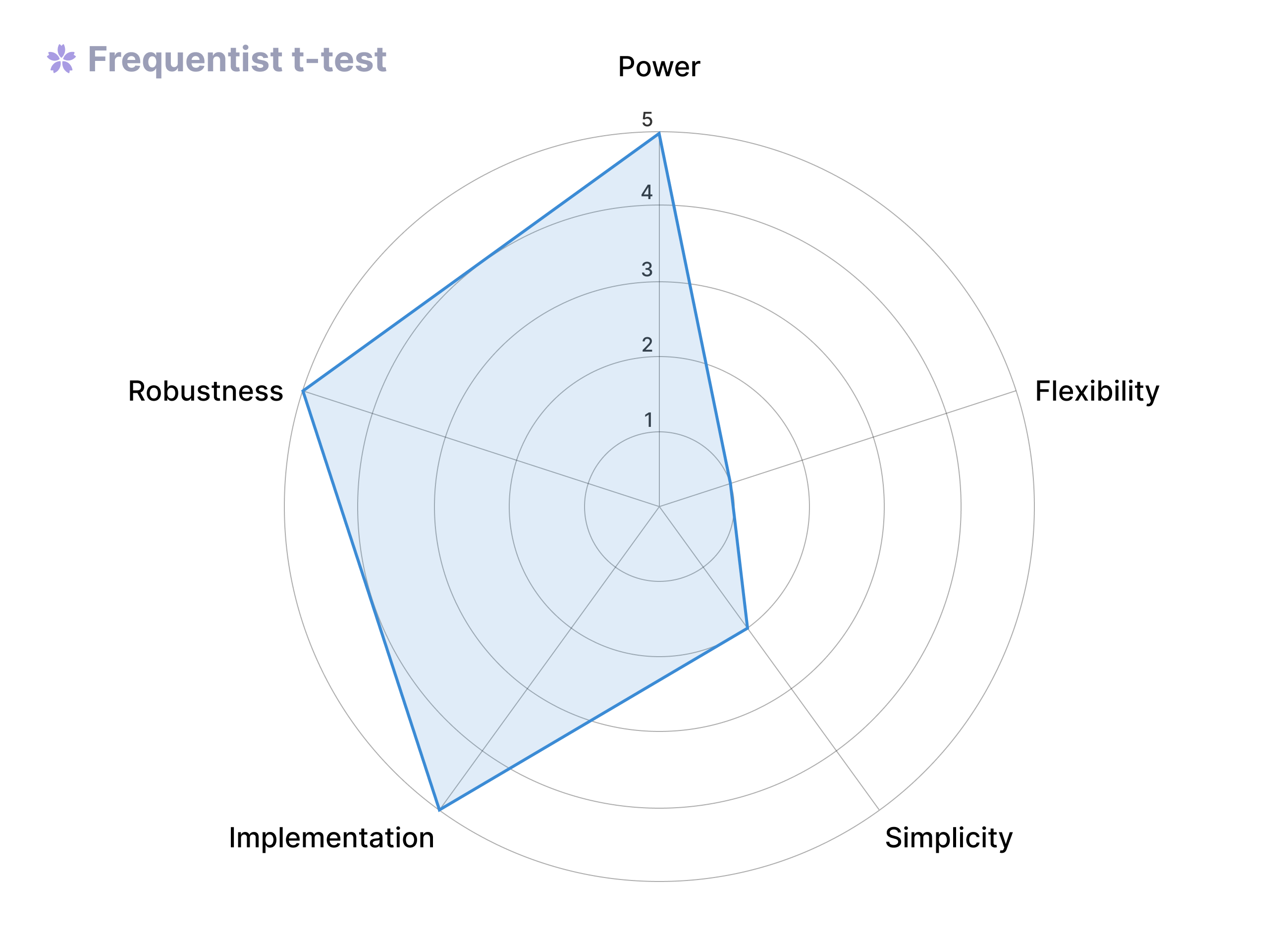
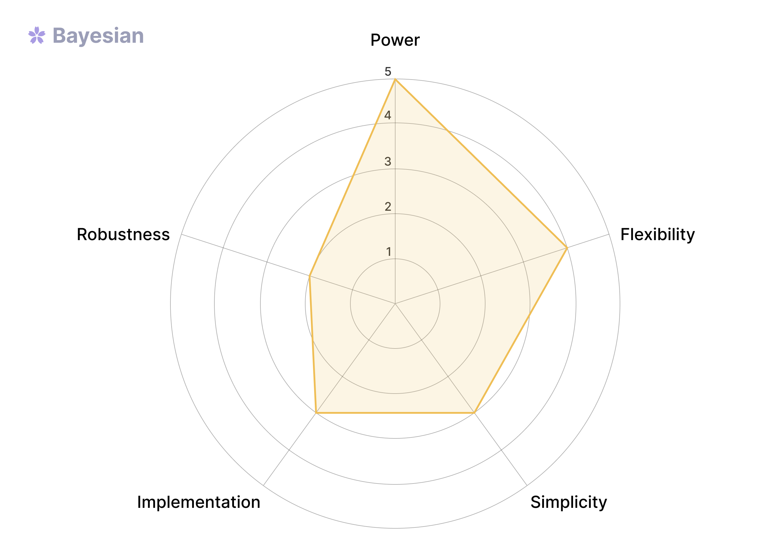
While there are many resources comparing statistical regimes, they tend to focus solely on statistical power. In this post, we argue that a more holistic comparison is beneficial, and analyze the five common statistical techniques along multiple dimensions (statistical power, intuitiveness, flexibility, robustness, and ease of implementation) in order to help you pick which methodology is the best fit for your use case.

This article was originally published on Eppo’s Outperform.

How we compared statistical approaches

In order to graphically compare these different statistical methods, we’ll evaluate them on a few key criteria:

Statistical Power

Statistical power quantifies how sensitive a method is to picking up differences in outcomes if they exist. Using a formal definition, it is difficult to avoid apples to oranges comparisons. Instead, when we refer to “statistical power,” we mean it more broadly: how much data must be collected to reach a particular specificity? An alternative way to think about power: if you run an experiment for X amount of time, how narrow are the confidence intervals (or credible intervals) at its conclusion?

For a deeper dive into comparing statistical power, Mårten Schultzberg and Sebastian Ankargren have written an excellent article.

Flexibility

Flexibility in this case refers to how well a method is able to adapt on the fly as more data becomes available. For example, if you realize the effect size might be bigger or smaller than you initially had anticipated, can you adjust the experiment’s runtime, or do you have to start from scratch?

Simplicity

This factor could also be described as the comprehensibility of the statistical method and its usage to a general audience. Proponents of Bayesian analysis, for instance, often prefer it for its intuitive definitions and explanations. Intuition covers both the ease (or difficulty) of setting up and running an experiment confidently (i.e., do you need an intimate understanding of statistics to use this method well?) and the ease of explaining the outcomes and results of your experiment to less-technical stakeholders.

Implementation

This factor refers to the technical effort required to run and analyze experiments using the method. Is it possible to quickly implement a particular statistical test? Are there standard packages available in popular programming languages? Does the approach scale well when analyzing many metrics and experiments?

Robustness

Finally, we look at robustness. Every statistical methodology is built upon assumptions that ensure validity. However, in practice, it is not always possible to guarantee that these assumptions hold. Robust methods can handle (small) violations in assumptions without completely changing the results. Some examples of assumptions that are often made when analyzing experiments:

• Normality of errors
• Multiple observations per user aggregated across time
• Non-stationarity across time

Comparing The Methodologies

Frequentist t-test

Hypothesis testing has a long and storied history, dating back to the classical t-test often taught in introductory statistics courses. This foundational method is the result of the combined work of Fisher, Neyman, and Pearson. In the classical t-test, you decide how much data to gather ahead of time (e.g., using a sample size calculator), then wait for all the results to come in before looking at the outcome to make a decision.

Pros of frequentist t-tests

• Achieves tight confidence intervals at the end of the experiment, resulting in high power to detect smaller effects.
• Strong and robust statistical guarantees; it is difficult to break the central limit theorem.
• Simplest to implement

Cons of frequentist t-tests

• Pitfalls like peeking may invalidate results, especially for less statistically savvy users
• Only valid with a pre-determined sample size; peeking is not allowed
• Choosing sample size in practice can be difficult as the effect size is unknown ahead of time

When to use the frequentist approach

• When we have very large samples. If we are operating at a scale where runtime is fixed (e.g., at a week or two), and we select the fraction of users to enroll in an experiment to be powered at that fixed runtime — think of organizations on the scale of Meta
• When we care about specific knowledge over the basic decision (i.e., if we care about having the best possible understanding of the actual effect size, we will want to have the tightest confidence intervals possible at the end of our experiment)
• When we can decently predict expected effect sizes (e.g., you have run similar experiments previously), since we need to choose a Minimum Detectable Effect to calculate your sample size
• When all teams involved in the experiment have the knowledge and discipline to not peek at the experiment or act early before the fixed sample size has been reached

Sequential testing

In the 1950s, sequential tests began to gain popularity, particularly in the medical field. One reason is that they allow for adaptability to the effect size being studied. For example, if there is uncertainty about how effective a drug is, a cure rate of 80% could be easy to detect quickly, but we wouldn’t want to discard smaller effects. Even if a drug is only effective for 20% of cases, that may still be very important for an otherwise incurable disease, but it would take much longer to detect. It would be unethical to continue providing patients with a placebo when we know a drug is effective. However, we also do not want to conduct the experiment with too short a duration, as this would result in reduced statistical power and make it difficult to detect smaller yet clinically relevant effects.

Group sequential tests

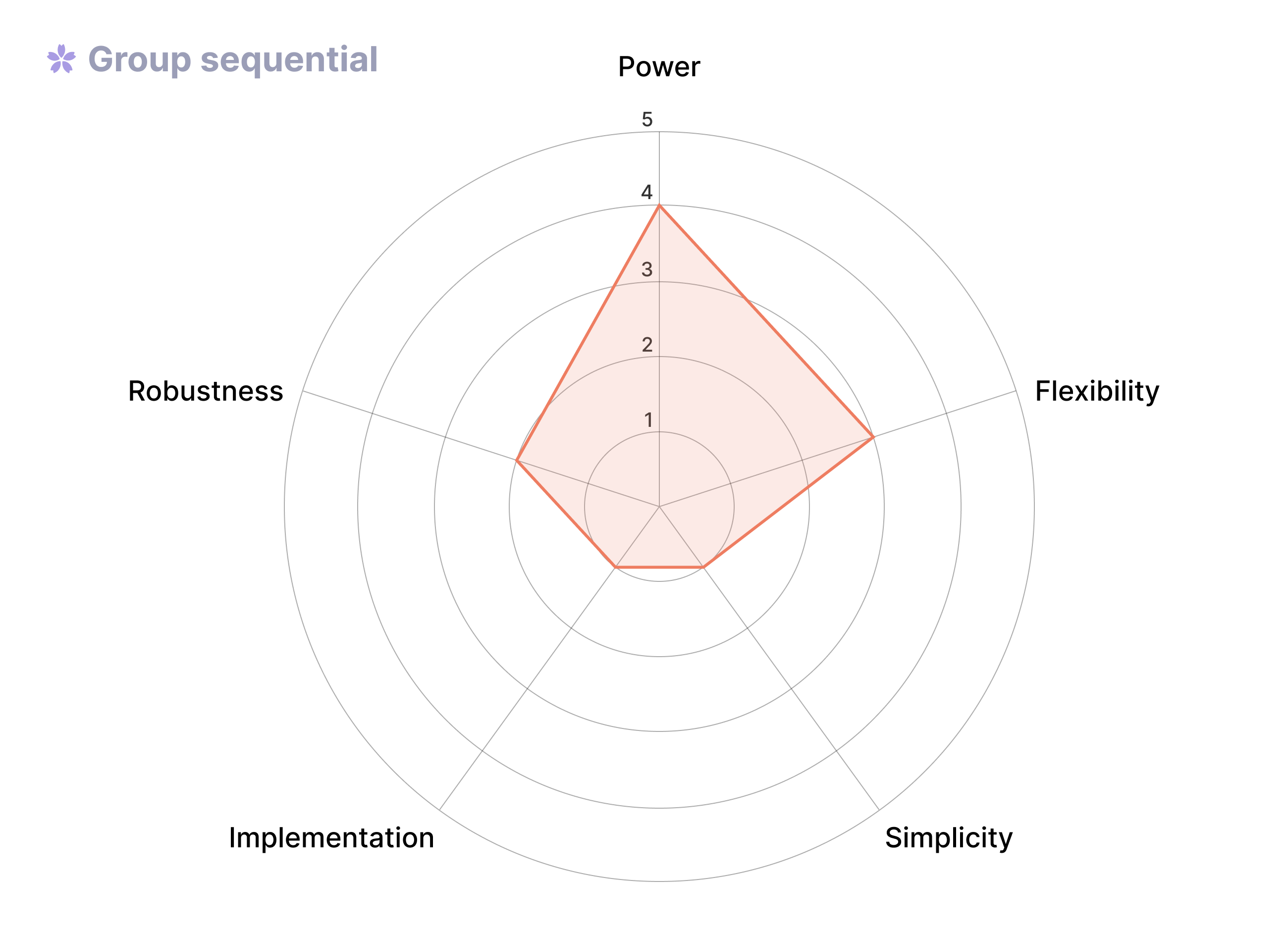
Group sequential testing plans for experimenters to make a number of interim analyses, or “peeks,” which are fixed in advance in both quantity and frequency. Group sequential tests have become particularly popular in the medical field and have also recently seen a surge of interest in industry, particularly at Spotify and Booking.com.

Pros of group sequential tests

• Allows for early stopping of experiments if effect sizes are large enough
• Leads to relatively tight confidence intervals by limiting the number of peeks, resulting in the highest-powered version of sequential tests

Cons of group sequential tests

• Hard to implement and code, with few open source available packages (recently Spotify released the Confidence package for Python, which includes a group sequential implementation ported from R)
• More work to do in advance of running the experiment since we now also need to select how and when to peek ahead of time The limited number of peeks may lead to a confusing user experience for teams following along (e.g., when results only update once a week) Relies on strong assumptions (iid observations, stationarity) that often do not hold in practice (more on this on the Spotify engineering blog).

When to use group sequential

• For experienced teams who want to leverage an optimal sequential test and don’t need to worry about impatience from stakeholders if peeks are only planned e.g. every week
• Important (or costly) experiments that are under the supervision of a highly trained statistician (that is why they are so common for clinical trials). In this case, you value the extra flexibility to stop early compared to the t-test, and do not mind the additional complexity.

Fully sequential tests

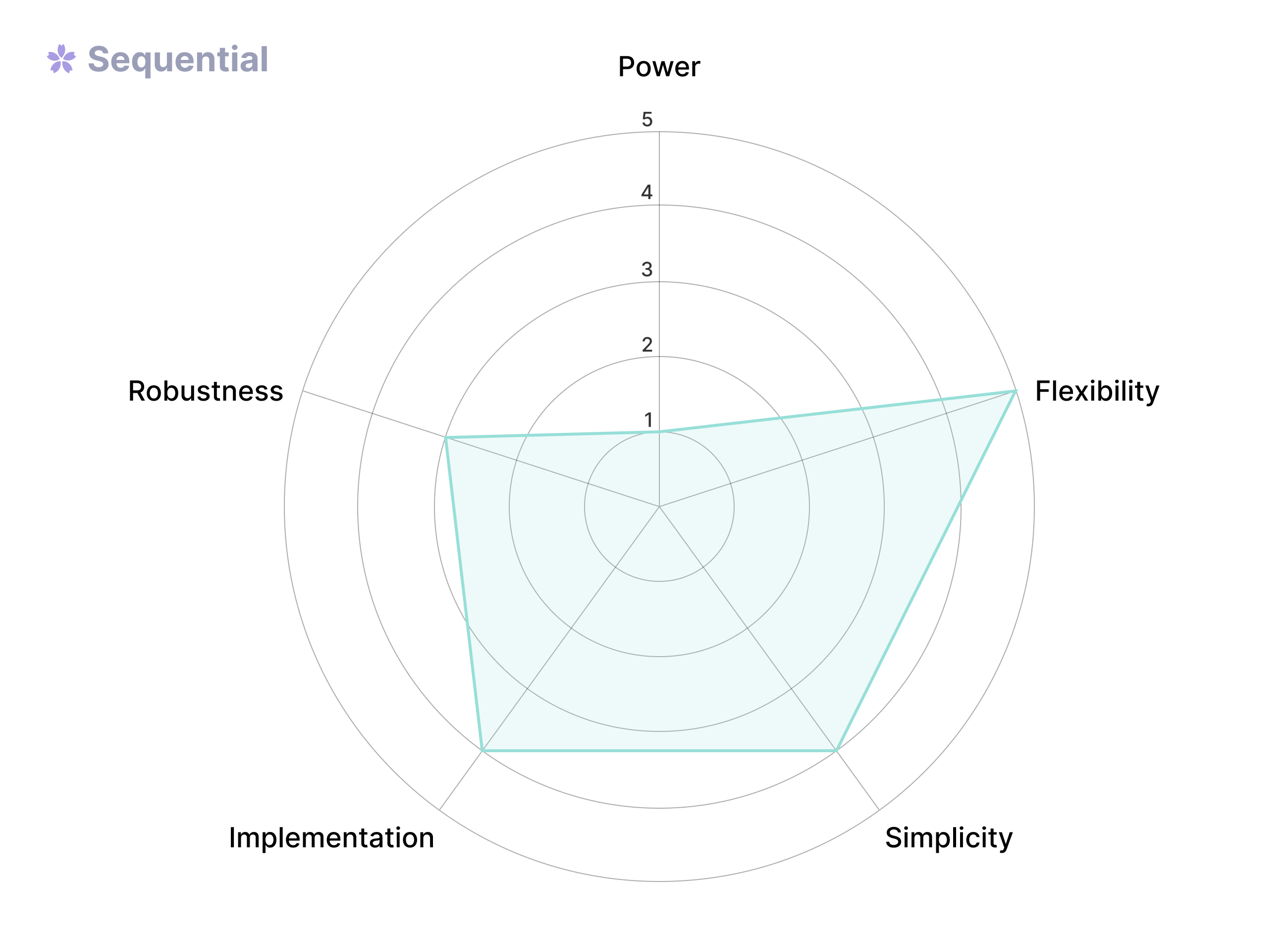
Fully sequential testing, on the other hand, allows the experimenter to stop at any point – no need to pre-determine your cadence and number of peeks. This method has gained more popularity in tech circles in recent years due to the data revolution, as we can now collect data continuously.

Pros of sequential tests

• Easy to set up, easy to use, and requires little oversight to run at scale
• The statistical guarantee is quite robust: it is not easy to break guarantees
• Most flexible: can end experiments early or decide to run the experiment longer
• No need to rely on a power calculation
• Can quickly detect large deviations in a metric (in both positive and negative directions)

Cons of sequential tests

• Experiment runtime is worse when there is a small effect or no effect at all
• Related to the point above, the confidence intervals at the end of an experiment are quite a bit wider compared to alternatives.
• While confidence intervals are always valid, the point estimates of early stopped experiments are more biased. This makes sequential tests less appropriate when the main goal is to learn about effect sizes versus making a decision quickly.

When to use sequential tests

Fully sequential methods are a good default when scaling up experimentation across teams less experienced with statistical analysis. There are no prerequisites to designing each incremental experiment, and the linear progress of the p-value makes it nearly impossible to misinterpret. It is also good at making fast ship/no-ship decisions with good statistical guarantees. That is, when making a quick decision is more important than understanding the precise impact. In this sense, it is the opposite of the classical t-test.

Hybrid sequential tests

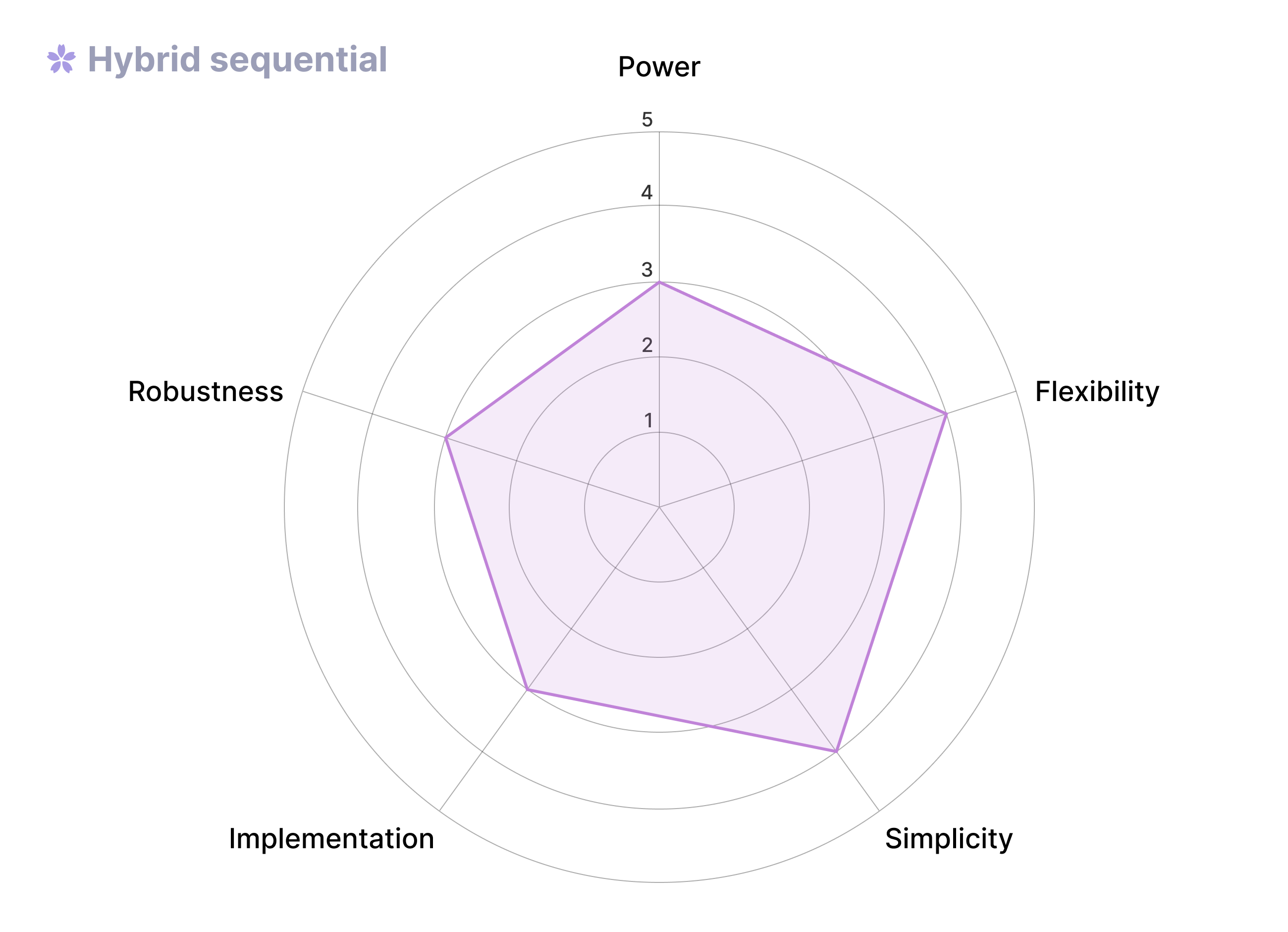
Because sequential tests generate a sequence of tests (or confidence intervals), rather than a single one in the case of a t-test, there is no single optimal “boundary” along the sequence. Instead, the experimenter has to choose where to concentrate statistical power. Particular choices for group sequential tests carry names, such as the O’Brien-Fleming test and Pocock test, while fully sequential methods usually have hyper-parameters one can set. More custom forms of customization are also possible. For example, it is possible to combine a fully sequential test during the experiment with a t-test at the end of the experiment period, using $\alpha/2$ as the significance level for each. This combines the best of both worlds, while a union bound shows that statistical guarantees are still met. We call this the hybrid sequential method.

Pros of hybrid sequential tests

• Achieves confidence intervals at the end of the experiment that are almost as tight as those generated by the fixed test, resulting in much high power to detect smaller effects compared to the fully sequential test
• Can stop experiments quickly when there are large effects (either increases or decreases).
• Overall, this provides a balance of strong statistical power at the end of the experiment while still allowing the user to safely peek during the experiment

Cons of hybrid sequential tests

• Like a frequentist t-test, requires specifying experiment runtime ahead of time
• Early stopping still leads to an increase in the bias of point estimates, similar to the fully sequential test.
  • Some use cases for hybrid approaches are more specific: Ronny Kohavi, for instance, suggests performing one-sided tests for negative outcomes sequentially, allowing for early stopping in cases of bugs or large degradations (when the point estimate is of less interest anyways)
• It may be confusing when observed confidence intervals suddenly switch to a tighter confidence interval at the end of the experiment

When to use hybrid sequential tests

When you want to combine the benefits from the fixed t-test approach (namely, power at the end of an experiment) and sequential approach (namely, early stopping).

Bayesian analysis

Finally, there is the Bayesian standpoint on experimentation. While all the above methods are frequentist in nature, Bayesian hypothesis testing involves forming a prior belief and then updating it with data to create a posterior. This approach can be difficult to compare with frequentist methods, as the underlying philosophy is quite different. Whether you like or dislike Bayesian methodology is mostly a matter of taste (debates on frequentist vs. Bayesian epistemology and intuitiveness are a common manifestation of this).

Pros of Bayesian tests

• Can explain results in more intuitive language. Even academics often define the frequentist p-value incorrectly, and many business stakeholders prefer the intuitive “chance to be best” (or similar) conditional probability that Bayesian analysis seeks to define.
• Utilizing a prior distribution helps shrink estimates and ease problems with peeking, winner’s curse effects, and multiple testing.

Cons of Bayesian tests

• Statistical guarantees are not as clearly defined and strongly depend on the appropriateness of the prior
• Selecting an appropriate prior can be difficult and is less accessible to non-experts in Bayesian statistics
• Can be more challenging to implement and compute at scale for more complex models.

When to use Bayesian tests

Whether to use a frequentist or Bayesian approach often boils down to preference, but here are some other subjective reasons:

• When you have documented experience running many comparable experiments and can use that empirical data to set appropriate priors
• If you prefer having the ease of explaining results over the rigor of strong statistical guarantees
• In small sample setting (regularizes effects, avoids underpowered analysis) — an important note on one misinterpretation of this benefit: Bayesian statistics does not make it easier to detect effects in small sample sizes, rather it protects you from thinking you have a big effect in small sample sizes when in fact there is none. Note also that in this case using an appropriate prior is even more important.

Conclusion

As is often the case in both statistics and life more generally, there is no silver bullet when it comes to selecting frequentist vs. Bayesian vs. sequential statistical methodology for analyzing your experiment results. Which method is most appropriate depends both on the specific situation and is partially a matter of preference.

Interestingly, the choice to utilize any one of the methods on this list relies not just on the technical context of what is being tested and how your experiment is implemented, but also on the experimentation culture of the team running and monitoring experiments. The experience level of the experimenters and other stakeholders, familiarity with the definitions of key terms, and even basic preferences may make any of these methods more or less appropriate.

For experimentation to drive stronger decision-making, tests must be both run and communicated well. These are challenges we’ve thought a lot about when designing the UI of Eppo’s experiment results and reports for each statistical method. If non-statisticians struggle to look at and understand the results, it will be tricky to grow an experimentation culture – regardless of how optimal your method is.

• Are bandits actually a good substitute for experimentation?
• And how do we know when to use one approach over the other?

Let’s take a closer look at experimentation (A/B testing) and bandits to better understand which approach is appropriate for each situation.

This article was originally published on Eppo’s Outperform.

Origins of experimentation and bandits

“You have to know the past to understand the present.” — Carl Sagan

Bandits and experiments (also called A/B tests or randomized control trials) may seem like two different animals, but they share a common trait: they’re both simple versions of a larger field of study. Experiments belong to the world of causal inference, while bandits fall under the umbrella of reinforcement learning. Understanding the origins of experimentation and bandits, and the goals of their respective broader fields of study is key to figuring out what each method excels at, and when it’s best to deploy them.

Causal inference

Causal inference is obsessed with answering “what ifs”: e.g. “would I be healthier if I take a daily multivitamin?” Of course, you could take the vitamins and see what happens; maybe you do actually feel healthier. But can we confidently ascribe this to the vitamins? You seem worried about your health more generally, and therefore might have improved your sleeping habits. On the flip side, what if you catch a cold at the gym the week after? You would not blame that on the multivitamins.

Ultimately, whether multivitamins are healthy is a difficult question to answer because we (unfortunately) only have one life and therefore can only observe one of the two cases; the fundamental problem in causal inference is that of missing values.

We can simplify this problem by taking two steps to arrive at experimentation. First, rather than asking whether multivitamin is healthy for one particular individual, instead we can look at the average over a population. While for an individual we can only observe one of the two possible outcomes, within a larger population we can see outcomes on both those who take multivitamin as well as those who do not. Second, instead of directly comparing people who take multivitamins to those who do not (maybe those who take multivitamins are more health conscious generally, and their healthier lifestyle, rather than the vitamins, is what impacts their health), we randomly assign only some to take the multivitamin. This ensures that we are comparing apples to apples, as the randomization makes sure that both groups are (probabilistically) equal.

Randomization simplifies the analysis by dealing with confounding factors (like a generally healthier lifestyle), but it does not compromise on inference. For example, what does it mean for a multivitamin to be healthy? Does it mean longer lifespan, or more energy, or less likely to get a cold? These are quite different metrics, but all can be analyzed through an experiment.

Reinforcement learning

The premise of reinforcement learning (RL) is rather different: here, an autonomous agent learns how to interact with a dynamic environment and find an optimal policy through interacting with it by taking actions and observing outcomes. The agent then improves the policy by taking into account what rewards it obtains from its actions.

In general, interacting with a dynamic environment is hard (e.g. think self-driving cars); multi-armed bandits reduce the complexity by making simplifying assumptions[^types of bandits]:

• The agent takes a single action out of a fixed number of options (arms)
• The agent observes the outcome (reward) immediately
• The environment resets and we repeat the process

The reduced action space and immediate rewards simplify the setting considerably, and help focus on the salient aspect of the setting: the trade-off between exploration (acting randomly and observing outcomes, nowadays better known as FAFO) and exploitation: selecting what seems to be the optimal action to maximize rewards.

Thus, the main difference between bandits and experiments is that a bandit tries to learn how to act optimally in a simplified setting during the data collection process, while in an experiment, the data collection process is only a means to run complex analysis afterwards.

So, concretely, what does it mean when your enthusiastic data scientist friend is advocating for using a bandit instead of an experiment? Rather than fixing the traffic split between variations ahead of time, they want to use the outcome from early users to adjust which variation gets shown to future users: if one of the variations in the experiment looks to be outperforming the others, we give that experience to more users (and to fewer users when it is underperforming).

Connecting bandits and experiments

So far, we have presented the bandit and experimentation settings as completely separate. However, we can connect the two using the “pure exploration bandit” (also known as best-arm identification problem). The pure exploration bandit shines another light on how the two settings differ, and this hybrid method could be exactly what you are looking for in special circumstances.

What is the pure exploration bandit? In the standard bandit setting, we care about the performance of the algorithm (or agent) as it interacts with the environment. This leads to the explore-exploit trade-off. As the name suggests, the pure exploration bandit does not care about performance during a learning phase. At the end of this learning phase, we judge the algorithm based on its final verdict on what the optimal arm is.

The setting is a clear hybrid between bandits and experimentation: we have the dynamic selection of which option to explore during the learning phase, similar to a bandit, and then the algorithm makes a single final decision on which everything depends, just like an experiment.

Let’s end this tangent with two more insights. First, when there are only two options, then the optimal algorithm in this setting is a fixed 50/50 split[^variance-assumption] — similar to the optimal experiment design but different from the bandit (which would favor the “best option”). Second, when there are more than two options, one way to solve this problem optimally is known as “successive elimination”[^successive-elimination]. This is an apt name: we try each option equally and eliminate options as we lose confidence that they are the best one.

Strengths and weaknesses

Now that we understand the origins of both experimentation and bandits better, as well as how they are connected, it is much easier to reason about the relative strengths of either approach.

Now versus future

Experiments are all about gathering data to make a final important decision where the cost of exposing (some) users (for a short period of time) during the experiment is outweighed by the benefits to all users “forever after.” Experiments focus on the future.

Bandits, on the other hand, care about the here and now[^forever-bandit]. Perhaps we’re trying to optimize website copy for our users for a Black Friday sale; we need to get the copy right for as many users as quickly as possible, and for the sake of this experience, there is no future beyond Black Friday itself.

More generally, bandits are much more appropriate when decisions are perishable, while experiments are better for evergreen decisions.

Impact estimation

When running an experiment, we fix the traffic fraction to each variation ahead of time. This means that all assignments are independent of outcomes, and thus unbiased estimates of the effects of each variation.

Bandit algorithms, on the other hand, adaptively update what fraction of users gets assigned to which treatment; otherwise, how could they exploit what they have learned so far? However, because the choices they make in the future depend on past outcomes, simple estimates of the impact of each arm have a negative bias.

Of course, in neither case we can completely escape biased estimation of impact: for both bandits and experiments the winning variation suffers from the winner’s curse, and this, in general, is difficult to correct for. That said, experiments generally lead to better estimates of impact for each variation.

Complexity

Bandit algorithms are very effective at optimizing for the simple loop discussed above: make a decision, receive feedback, rinse and repeat. However, the downside is that bandits are more brittle when it comes to complexities we often encounter in practice:

• There are time-varying effects (both seasonality, as well as newness bias); all best known bandit algorithms assume there are no such effects and can get easily tripped up.
• We care about multiple metrics, which often is the case. To make matters more complicated, we may have guardrail metrics; e.g. we might not care directly about an experiment improving page load times, but we also want to guard against page load time degradations. A bandit algorithm would require us to summarize all these metrics into a single number in order to work.
• Feedback is delayed; we do not immediately get to see whether the action we took led to a good or bad outcome and thus we have to wait until we observe the outcome before we can update the bandit.
• We want to provide a consistent experience to a user. The adaptive allocation of bandits makes it difficult to keep users in a single experiment across multiple sessions.

As the scenario becomes more complex, experiments become more attractive, as they are more robust and allow for us humans to add nuance to a decision.

Implementation and computation

When it comes to implementation and computing results, experiments have a clear leg up on bandits; in general, experiments only require flipping the same coin over and over, and analysis is naturally done all at once in a batch. This makes it (relatively) easy to get started with experiments.

On the other hand, bandits are sequential: they constantly update which action to choose next. In general, such sequential decision making is more tricky; and while some bandit algorithms can be converted to batch updating (such as Thompson sampling), this is not always straightforward (e.g. for upper confidence bound methods).

Use cases

News-headline optimization

My favorite use case for bandits is news headline optimization: suppose you work at the web division of the New York Times and need to put a title on every article. You could let the editor decide ahead of time (as is needed for the paper version), or, you could gather a few options and have a bandit algorithm figure out which leads to most readership.

It is a natural fit for the bandit scenario: a news article is only relevant for so long (perishable); a news outlet writes many articles and each is a distinct problem; it’s inefficient to have a human decision maker in the loop for each decision; and the feedback is immediate: did a reader open the article and read it? Finally, while understanding what makes for a good headline is undoubtedly useful, there is no need for a deep dive on a per headline basis.

Some other great examples for bandits are:

• An email campaign for Black Friday sales
• Optimizing thumbnails for products or movies

Sign-up funnel optimization

Because experiments can handle nuance much better than bandits, there are many more examples of companies successfully using experimentation, e.g. in two-side market places (like Airbnb, Doordash, and Uber) and recommendation systems (like Netflix).

To illustrate, let’s consider a common problem where experimentation is clearly more appropriate than a bandit: testing a new sign-up funnel.

This decision can be complex and have a big impact on business outcomes, and it usually involves many stakeholders. The decision criteria are difficult to specify, with both short and long-term metrics needing to be taken into account. Furthermore, it’s undesirable (if not impossible) to have potential users switch between two flows if they return to the funnel rather than completing it in one session. Finally, redesigning a sign-up funnel is a significant effort that shouldn’t be done frequently. Whatever the decision may be, it will likely remain in place for a while. Therefore, it makes sense to prioritize the future over the users in the experiment. All of the above point clearly to running an experiment over using a bandit to allocate users to sign up flows.

Conclusion

Both bandits and experiments help us make data-driven decisions, but their use cases clearly differ. To understand these differences, it is best to look at their origins in reinforcement learning and causal inference, respectively. This highlights the clear distinctions between the two approaches, with one often being superior to the other in certain situations.

Bandits are best suited for time-sensitive decisions with low complexity, such as news headline optimization, while experiments are more suitable for long-term decisions where there is a lot of nuance; a good example being an experiment on the sign-up flow. In practice, more often than not there is nuance one way or another, and this leads us to favor experiments over bandits, but in certain scenarios bandits are terrific.

Please let us know about your favorite experimentation and bandit use cases!

Footnotes

[^types of bandits] There are two distinct bandit settings: the stochastic bandit we are focusing on, and the adversarial bandit.

[^variance-assumption] This assumes equal variances of outcomes for the two variants.

[^successive-elimination] See this paper for a more formal description of the successive elimination approach.

[^forever-bandit] In theory, this is not true: you can run a bandit forever and indeed the whole reason a bandit explores is because it cares about making good decisions in the future. However, in practice we rarely run a bandit “forever”. You can think of an experiment as “explore during experiment, then exploit forever after making a decision”.

In experimentation, the p-value is the least understood and most misused concept, with both the most common and egregious error stating that the p-value is the probability that the null hypothesis is true. I certainly relate, as I quite often catch myself moments before making this mistake.

To better understand p-values, let’s go back to the fundamental definition of what constitutes a p-value. We can use it to construct a useless p-value. That is, a p-value that is useless in practice but pedagogically useful. We find many useful insights that help us understand not just the p-value, but also the statistical concept of power, and issues related to multiple testing and peeking.

Taking a step back, most of us have struggled with a mathematical concept at some point in our lives. I definitely have, and usually it’s been because I was looking for some magical insight that would make me understand it all. It’s easy to be stuck “waiting for the epiphany”, unable to make any progress.

However, understanding often comes not from waiting for the epiphany, but rather giving up on the search for that special insight and rather just take a definition at face value and getting your hands dirty (or more likely: a piece of paper dirty). By playing with the definition, creating examples and counter-examples, we can start to build intuition until we are no longer intimidated by this seemingly unintelligible concept or daunting definition.

This article was originally published on Eppo’s Outperform.

Fundamental definition

To keep things semi-formal; consider the classical frequentist hypothesis test. We are testing a null hypothesis (could be anything: that the mean is zero, that there is no effect on revenue in an A/B test, etc.) against an alternative. Then the most fundamental definition of a p-value (sometimes referred to as a conservative p-value) is:

Definition of p-value. The random variable $p$ is a p-value if, under the null hypothesis, $P_0( P \leq p ) \leq p$. That is, $p$ has a super-uniform[0, 1] distribution.

Let’s unpack this definition. First, a p-value is a random variable; in frequentist statistics, the underlying parameters are fixed (e.g. whether the mean is 0, or 1, or $e^{i\pi}$), and the data is a random variable. Since a p-value is a function of the data, it also is a random variable. This makes sense: if we were to repeat an experiment, we collect new data which leads to a different p-value.

Let us look at some examples of super-uniform random variables to build intuition:

• The constant 1 is super-uniform — it’s always larger than a draw from a uniform random variable on [0, 1].
• The uniform distribution on [0, 2] is super-uniform. One way to see this is as follows: if $U$ has a Uniform[0, 1] distribution, then $2U$ has a Uniform[0, 2] distribution, and $U < 2U$.

Finally, note that this definition places no conditions on what happens to a p-value when the null hypothesis is not true. Officially, a p-value can take any value when the null hypothesis is not true, but in this freedom ultimately lies our power to create useful p-values. We will return to this shortly when we talk about (statistical) power.

The useful useless p-value

Armed with the fundamental definition of a p-value, arguably the simplest p-value is the constant $1$. Clearly, this satisfies the definition of a p-value, but it is too useless even for us.

Instead, meet $u$, our useful useless p-value. $u$ is a Uniform[0, 1] distributed random variable and therefore also trivially satisfies the definition of a p-value. We can reject the null hypothesis whenever $u < \alpha$ and ensure a type 1 error rate of $\alpha$ (that is, falsely rejecting a true null hypothesis).

Now that we have gotten introductions out of the way, let’s focus on understanding why $u$ is both useless and useful.

Useless

The guarantee of our new p-value is rock solid. Of course, under the null hypothesis, the probability that $u$ is less than 0.05 is exactly 0.05, which matches the guarantee we are looking for. However, this is of course also true when the null hypothesis is false. Therefore, we have a low false positive rate (as required), but also a high false negative rate.

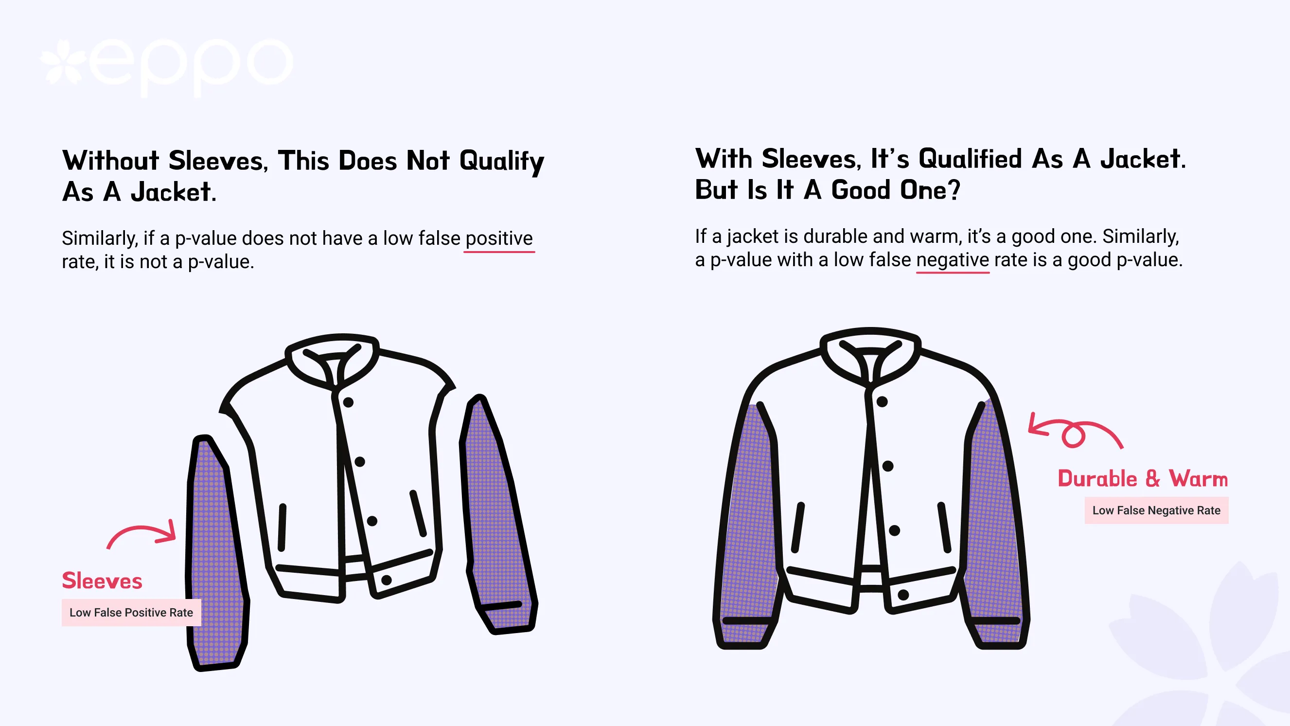
We can create an analogy with a jacket: it needs to have two sleeves to qualify as a jacket (otherwise, we would call it a body warmer); but a good jacket is warm, waterproof, and durable. Similarly, a p-value needs to have a low false positive rate, but to be a good p-value, it also should have a low false negative rate. Statisticians refer to this as “power” (power = 1 - false negative rate). In practice, that means that whenever the null hypothesis is not true, a good p-value is as small as possible. So, $u$ is definitely a p-value, but it is a useless p-value because it has low power.

Useful

While it should be clear why $u$ would not make for a useful p-value in practice, it does show its value in explaining important statistical concepts. Let’s dive into them.

Post-selection inference

⚠️ Statistical jargon alert! ⚠️ Post-selection inference sounds intimidating, but it really shouldn’t be. In statistics 101 we learn that the proper way to run a hypothesis test is: “make up a story” and then “use the hypothesis test to verify or disprove your story”. Post-selection inference turns that upside down in a subtle way: “first use data to find a result”, and then “make up a story” — it turns out the latter is a primary cause of headaches for statisticians.

Let’s use our $u$-value to make this more tangible. Suppose you run a speculative experiment; you think it’s pretty likely there is no effect. We generate our $u$ value and, lo and behold, $u = 0.023$; hurrah, we can reject the null hypothesis! Do you feel good about your experiment? Do you believe that you are one step closer to your Nobel prize?

No… but, nonetheless, something interesting happened; our $u$-value controls type I error: we know it rarely rejects the null hypothesis when its true. With a $u$-value less than $0.05$, we can actually reject the null hypothesis, and yet not feel any better about ourselves, nor our experiment. Why?

It is because we realize rejecting the null hypothesis was a random fluke — in this particular case we are pretty certain we are committing a type 1 error[1]. This highlights a general truth about p-values that is easy to forget: it is the p-value that is the random, not the truthiness of your hypothesis (and if you do not like this: congratulations, you are a Bayesian 🎉).

Once the p-value is generated, there are no more probabilistic statements to make.

Our useless p-value illustrates clearly that any statements such as

• “the p-value is the probability the null hypothesis is true”, or
• “the p-value is less than $\alpha$ and thus the probability that the null hypothesis is true is less than $\alpha$

make absolutely no sense from a frequentist perspective (and again, we’re doing frequentist statistics here). And this naturally brings us to the next concept to explore.

Underpowered studies

Even the best statistical methods are beholden to the quality of the data: one issue that plagues both academic studies as well as experiments in industry are underpowered studies: this refers to the setting where we have not gathered enough data to be able to confidently detect meaningful changes, even with state-of-the-art statistics: there is more noise than signal.

At first sight, the issue is not apparent: the p-value controls type-1 error no matter what, so what is the big deal?

When there is not enough data to detect a signal in the noise, our p-value is basically a uniform random variable whether or not the null hypothesis is true or false. That is, any p-value becomes a $u$-value. And in the previous section, we discussed the issue with that arises with this: a rejection of the null hypothesis by a $u$-value is meaningless. It does not help us build confidence in our alternative hypothesis at all.

For underpowered studies, every p-value looks like a $u$-value.

The problem with underpowered studies is that they are “dead on arrival” — whether or not we end up rejecting the null hypothesis makes no difference, in either scenario we have not gained any insight. Of course, when we do end up rejecting the null hypothesis, it may not be so apparent that we are at high risk of making a type 1 error as with our $u$-value. [2]

Multiple testing

What is the probability a coin comes up heads? A simple answer would obviously be 50%; if you are a little more paranoid you might ask: “is the coin unbiased?” before answering (let’s assume it is). Still, this misses a salient aspect of the problem: how many coins are being flipped? Indeed, for a single coin it is 50%, but if I were to flip 2 coins, it becomes 75%.

The same is true when we are running multiple hypothesis tests (e.g. when looking at multiple metrics in an experiment, or look at single metric for multiple segments). When we generate 20 $u$-values, with probability ~64% at least one of them will be less than 5%. We have a tendency to look at the smallest p-value, as that one corresponds to the “most significant” effect, which lands us in hot post-selection-inference waters. But this is now exacerbated by the fact that even some of our useless $u$-values will be small.

The natural way to correct for this is to demand even smaller p-values when you run multiple tests — rather than being significantly smaller than a draw from a uniform distribution, you now want your p-value to be significantly smaller than the smallest out of many uniform distributions. Put differently: the more p-values we generate, the more strict we should be before rejecting null hypotheses (which can be made more precise). This increases the burden to find a sufficiently strong signal within the noise and hence makes it more likely we are running an underpowered experiment. [3]

When running multiple tests, it is important to both be more strict in rejecting null hypotheses, as well as worry more about underpowered experiments.

Peeking

Finally, let’s cover the peeking problem. Now that we have covered multiple testing, this should be easy. We return to our $u$-value, but change the scenario slightly. Suppose, rather than gathering the data and then generating a single $u$-value (by now you might be sufficiently comfortable to skip the gathering data part), instead we generate a new $u$-value every day during the course of a month of “data gathering”. r/whatcouldgowrong? Clearly, the peeking problem is a multiple testing problem; again, with a probability of about 64% we will see at least one $u$-value less than 0.05 during the first 20 days of our experiment. Thus, if we reject the null hypothesis the first time we see a “statistically significant” $u$-value, our false positive rate will be much larger than 5%. Of course, this problem goes away when we discard all but the last $u$-value (that is, do not peek). The other option is to be more conservative in rejecting null hypotheses, but unfortunately that also means that we have to worry about Mr. Underpowered — the field of sequential analysis makes this more rigorous.

Conclusion

u = random.random() is a valid p-value. While you probably want to avoid its use in practice, I hope this post has convinced you that it is a very useful pedagogical instrument that helps understand frequentist hypothesis testing. In particular, we now understand its more subtle and dangerous aspects: post selection inference, underpowered studies, multiple testing, and peeking. Most importantly, hopefully now it is now easier to avoid misrepresenting p-values with any kind of probabilistic meaning.

Finally, note that we can trivially adapt this article to be about the Useful Useless Confidence Interval instead. This is left as an exercise to the reader.

Footnotes

[1] We have to put on our Bayesian hat to make this more precise, something I’m trying to avoid in this particular post.

[2] For a deeper dive and a Bayesian perspective, I recommend Beyond Power Calculations: Assessing Type S (Sign) and Type M (Magnitude) Errors by Andrew Gelman and John Carlin

[3] There’s an interesting tangent here: suppose I generate 100 (valid) p-values simultaneously and I tell you that 20 p-values less than $0.05$. Then you know something interesting must be happening even without knowing anything about my statistical procedure. On the other hand, if I tell you that that there are only about 5 rejections, you are none the wiser: maybe there are no effects, or maybe I’ve been generating $u$-values and a more powerful methodology for generating p-values would have found more interesting results.

Note: the plenary talks should be posted on Youtube in the next few weeks, at which point I will update this post with links. The figures used in this post are taken from the published work by the respective authors.

Jake Hoffman on the effects of UX on understanding of uncertainty

Jake Hoffman kicked off the conference with an important and often undervalued aspect of experimentation: the user interface really matters. Starting from the “inference” versus “prediction” views popularized by Breiman, he showed that even expert’s interpretation of effectiveness of a drug in an experiment depends a lot on whether one uses standard error of the mean (underestimates variability and hence leans effective) or the standard deviation of the sample (leans ineffective).

It is an important reminder that while we tend to nerd out on the mathematical problems, we cannot forget about the user experience; we need to make sure results are accessible and empower everyone to make good decisions, not only those with a PhD in Statistics.

Interference

It’s clear that interference is clearly one of the most important open issues in experimentation, and more and more people realize how it is affecting their experiments. For those less acquainted with this problem: interference occurs when treatment of one subject in the experiment affects outcomes of other subjects, for example due to a network structure (video chat is only valuable if your friends also have video chat) or a two-sided market (if you book a room, then it is no longer available for someone else). The good news is that there is a lot of exciting research happening in this area.

Ilan Lobel on leveraging shadow prices

Interference can take many forms, and is often difficult to model. However, Ilan Lobel argues that the problem can be cleanly modeled in matching markets where a platform has strong control over the matching process (think Uber/Lyft). Namely, the shadow prices of the optimization problem can be used to correct for the bias introduced A beautiful linearization argument both shows the issue from using naive estimation of the average treatment effect (HTE) and how shadow prices address this.

At Stitch Fix I worked on both improving matches between clients and inventory using shadow prices, and on correcting for interference in the experiments we ran, but we never realized the connection.

The full paper is on Arxiv.

Kris Ferreira on human algorithm collaboration

In a fantastic plenary talk, Kris Fereirra discussed her quest to understand how decision makers are interacting with algorithms to make better decisions, and what pitfalls they fall into. By decomposing information into a public part, accessible by both decision maker and algorithm, and private part, only accessible to decision maker, she shows that decision makers struggle to understand when the algorithm provides strong predictions versus when they should rely on important private information to overrule the suggestions by the algorithm.

Instead, decision makers tend to use a convex combination of their own prediction and the algorithm’s suggestion independent of the quality of the quality of the algorithm’s prediction on a particular task. This leads to suboptimal decision both when the algorithm is correct as well as when it is wrong.

There is clearly growing interest in understanding human-algorithm interaction, and I am curious to see how this area develops in the coming years.

Kelly Pisane on unbiased impact estimation

High on my list of best talks was Kelly Pisane from Booking.com She discussed how to go about obtaining unbiased impact estimates from statistical significant experiment results. The talk stands out because it demonstrates clearly that sometimes simple and practical suggestions trumpet complex mathematical modeling.

Every experiment platform faces a post-selection bias problem: statistically significant effect estimates have an upward bias, but it is difficult to understand the magnitude of this bias. Rather than trying to correct for this mathematically, we can do the following: after making a decision, split the remaining users in the control group and use data from that “experiment” to get unbiased estimates of the treatment effect. We avoid the issue that users may already have been exposed to the winning treatment. Furthermore, it often takes some time for engineers to roll out the winner anyway, so you might as well run this second, impact, experiment. Even if you are underpowered to understand the impact of a single experiment, the data can still be used in aggregate across experiments to understand the true impact of experiments. Clever indeed!

Sequential testing

There is clearly a lot of momentum in both academia and industry on sequential testing, with an entire session dedicated to it at the conference. If you are less familiar with sequential testing: unlike classical frequentist methods, this methodology allows for continuous monitoring and adaptive decision making with strong statistical guarantees.

Netflix is heavily invested in sequential testing, with multiple talks, but also Microsoft and Adobe are adopting the sequential paradigm. That said, the sequential framework has pros and cons and does not fit every use case. It will be very interesting to see how this space develops in the coming years

Michael Lindon on sequential testing procedures for regression

It is hard to pick a particular talk from a session full of great content, but personally I really enjoyed Michael’s talk on extending sequential procedures for regressions; this enables us to combine sequential analysis with pre-experiment covariates and linear regression to reduce variance and thus speed up experiments.

Two aspects of this talk stood out to me in particular.

1. It is often easy for research to lean theoretical, but here the practical use case is extremely obvious: adjusting for pre-experiment data often speeds up experiments substantially.
2. The approach by Netflix is similar but also quite distinct from the way we at Eppo model this problem.

The latter is indicative of a broader phenomenon that stood out at the conference: we all have different approaches to the same problems and that makes it particular valuable to come together and be inspired by each other’s work.

Finally, worth mentioning is the call out by James McQueen that in practice it is very rare to observe a single outcome per user. Instead, we observe a sequence of events from which we construct an outcome that evolves over the duration of an experiment, but this often gets ignored in theoretical work on experimentation. Having struggled with this myself, it is great to see this problem being more broadly.

The full paper is on Arxiv.

Hamsa Bastani on COVID prevention in Greece using Bandits

When it comes to bandits, everyone seems to agree on two things:

1. They are beautiful to study from a theoretical standpoint
2. But in practice they are not used all that much due to a variety of complications

Hamsa demonstrated that bandits can be powerful in practice, even under challenging circumstances. Picture the setting: it is Spring 2020, the pandemic has just started, and in Greece, the tourist season is approaching rapidly. Since tourism accounts for 25% of GDP, Greece literally cannot afford to remain in lockdown and decides to open borders for tourists. How do you keep the public safe when you expect 30k to 100k tourists to arrive every day, while you only have a limited capacity of 8k daily PCR tests that have a 2-day turnover time. Furthermore, the rate of COVID infections flares up in different countries across time so the testing results are only useful for a short period of time before becoming outdated. How can you allocate the limited number of tests in a way that minimizes the number of infected tourists entering the country? Hamsa and team’s answer: use a contextual bandit.

Lo and behold, it worked and the team caught almost twice as many infection than random sampling would have. Hamsa demonstrates there is hope for the practical applicability of bandits, and likely saved affair number of lives in the process.

The full paper is published in Nature.

John Cai on heterogeneous treatment effect estimation

Another big topic at CODE was understanding and estimating heterogeneous treatment effects (HTE), with clear applications in industry illustrated by talks from Snap, Netflix, and Meta. Automatically finding segments of users for whom a treatment works particularly well, or poorly, has clear applications but is also a thorny problem that is far from solved.

John Cai from Snap gave an overview of Snap’s approach to HTE, bridging the gap between theory and practice: first by evaluating the effectiveness of testing whether HTE exist in the first place. If there are no heterogeneous effects, then a reasonable assumption is that the variance of control and treatment are the same. This reduces the problem to testing the hypothesis that the variances are equal.

If we do detect a difference in variances, then we can focus on finding dimensions that contribute most to heterogeneity in treatment effects by decomposing the total treatment effect variation into explained and idiosyncratic variation. All of this was demonstrated using an actual experiment the team ran at Snap.

Wrapping up

It is clear that interest in experimentation is growing rapidly, and we are only scratching the surface on problems practitioners face. In particular, I expect there to be a lot more work on interference, sequential testing, heterogeneous treatment effects, and understanding long term outcomes. But as we nerd out on these problems, we should also keep the UX in mind: we cannot just solve the mathematical problems, we also need to make solutions accessible to the non-expert so they feel empowered to make better decisions.

If you also attended CODE, let me know what your highlights are. If you did not, hopefully this inspires you to visit Boston next year; the weather was surprisingly great!

The Great Debate

When you are building an experimentation platform, it’s impossible to avoid the debates between frequentist and Bayesian approaches to hypothesis testing. Ardent supporters on both sides espouse the benefits of their approach, but when the debate has been raging for decades, and between the most famous and brightest statisticians, it’s no surprise there aren’t any easy answers.

An oft highlighted issue of the classical frequentist approach is that of the peeking problem: with modern tooling, it’s often easy to monitor the results of experiments while collecting data. However, the frequentist guarantees break when you peek at experiments, leading to an inflated type I error rate: you end up claiming there is a difference between variants far more often than you want to in the case both variants in fact have the same outcome distribution. On the other hand, Bayesian supporters often highlight that the Bayesian approach does not suffer from the peeking problem, claiming that this is one of the benefits of using a Bayesian testing regime over a frequentist one.

Statistics is often more subtle than it first seems, and so we have to wonder: is this too good to be true? Famous Bayesian statistician Philip Dawid wrote a fantastic paper in the 90s: “Selection paradoxes of Bayesian inferences”, shared to me by Steve Howard, that I highly recommend you read. It’s fairly accessible, both in that there is no paywall, and that the reasoning is easy to follow. In this work, he introduces what I would like to call the “Bayesian imposter”: someone who claims the benefits of the Bayesian approach, while actually doing frequentist analysis.

Let’s put this in an experimentation context. Before we do however, I want to note that this post is not about choosing sides: both frequentist and Bayesian approaches have their merits, and shine in different ways. Rather, the work of Dawid helps us to understand and appreciate the subtleties in this debate.

The experimentation setting

First of all, let’s get on the same page regarding what an experiment is; we will keep it high level and consider the most basic setting; it is all we need. Consider we want to test a new variant: treatment, versus the status quo: control, and we would like to figure out whether treatment is better than control according to some metric we care about. We resort to some statistics to help us figuring this out: We randomly assign subjects to either treatment or control, and measure the outcome on said metric. Now we use some statistical method to compare the two variants, e.g. by comparing the means using a T-test (frequentist) or comparing the posteriors by combining priors with a likelihood (Bayesian).

Frequentist versus Bayesian hypothesis testing

Before diving in, let us briefly recap the differences between frequentist and Bayesian hypothesis testing.

In the frequentist setting the underlying parameter fixed, while the observed data is considered as the random variable. Thus, the frequentist thinks about guarantees on their inference methods through considering repeated draws of data. For example, a confidence interval is a function of the data (thus also a random variable), with the underlying idea that as we generate data, and hence confidence intervals, over and over, most times the generated confidence intervals contains the parameter of interest. But this has the unintuitive downside that a frequentist cannot give any certainty about a particular set of observations.

The Bayesian perspective flips this around: you are handed a set of observations, clearly those are fixed. What you do not know is the value of the underlying parameter, so let’s consider that the random variable. We encode our beliefs through a prior distribution for said parameter, and then combine that with the likelihood of observing the data given the parameter to form a posterior distribution. Now the posterior distribution allows us to reason about this particular outcome: conditioning on the data is not a problem, because inference on the parameter is already conditioned on the data!

The last point is often quoted as one of the main benefits of the Bayesian approach to experimentation. With the classical frequentist approach sample size needs to be fixed up front (we cannot be adaptive to data). If we ignore this and decide whether to continue collecting data based on what we have observed so far, or are ready to make a decision, we can dramatically increase the risk of a false positive. This is different for in the Bayesian case, we can be adaptive, and make a decision at any point: do we keep gathering more data, choose the treatment variant, or the control variant. This follows from your elementary probability class: from the Bayesian perspective, the data is fixed (a constant) and only the parameter we are interested in is considered a random variable. Conditioning on the data (a constant) does not impact results.

Dawid’s paradox

But is it really so black and white? Dawid, a well known Bayesian statistician, posed the following paradox in the paper mentioned above: The Bayesian approach sounds great: we can be adaptive to the data, while the frequentist cannot. But now consider a Bayesian that uses a non-informative prior (or flat) prior: a prior for which every outcome is equally likely. It is easy to see that when using such a non-informative prior, the frequentist and Bayesian approach lead to the exact same results: the Bayesian approach multiplies the likelihood with the prior to get the posterior (modulo normalization). If the prior is flat, then we are multiplying the likelihood by 1. Hence, our inference is based only on the likelihood – exactly the same likelihood the frequentist is using!

But now the adaptivity is a bit odd: how can it be fine to be adaptive (or peek) when using the Bayesian approach, while the frequentist is stuck waiting to collect all their data, despite the two approaches leading to exactly the same results?

Resolving the paradox

The culprit is clear: it is the flat prior that causes the Bayesian posterior to be the same as the likelihood on which frequentist analysis is based. As usual, there is no free lunch: the Bayesian approach has not magically solved the issue of peeking for free. Rather, to solve the problem posed by peeking, we need to solve the problem of the prior: Bayesian analysis works when the prior works. David Robinson demonstrates the same point using simulations.

Adaptivity, or the ability to peek, is very powerful and the Bayesian approach is far simpler than the frequentist alternative of sequential testing. But powerful results often require strong assumptions; in this case the need for a well-chosen prior.

In particular, when we are unsure what prior to choose, the suggestion to use a weak prior is much more common than to use a strong one, and this makes sense: in the small data regime, a strong prior can dominate the posterior, which is undesirable especially when we do not feel strongly about the strong prior. But the discussion above reveals that it is a balancing act: both weak and strong priors have downsides and hence carefully finding the correct balance is unavoidable.

Take-away

Bayesian and frequentist approaches and guarantees are fundamentally different, but under certain conditions, they lead to exactly the same results. Dawid demonstrates clearly that this creates a paradox: when results are the same, approaches cannot have fundamentally different guarantees. This is where the Bayesian imposter comes in: to truly enjoy the benefits of a Bayesian approach, one needs to carefully think about what prior to use, otherwise, the experimenter might just a frequentist in disguise, and be ignorant of the risks that poses to the validity of their statistical claims.

More generally, when the experts have been debating the respective merits of frequentist versus Bayesian approaches, it must be true that one cannot be clearly better than the other: then the debate would have been settled a long time ago. When you experiment as a Bayesian, make sure you think carefully about your prior, or you might well be a frequentist without realizing it!

The goal is to create a character level language model using a simple RNN following the approach by Andrej Karpathy’s 2015 blog post “The Unreasonable Effectiveness of Recurrent Neural Networks”, but focus on Jax rather than creating an unreasonably effective network. That is, given a reasonably sized text, say a book, we want to create a model that generates content one character at a time. We will find that it is relatively easy for the simplest of RNNs to learn how to string together a few words using a small network and few training epochs.

We will assume a basic familiarity with Jax. You can find the code on colab, and I am by no means a Jax expert, so feel free to reach out with comments and suggestions.

Flax

There are a few libraries built on top of Jax that help with creating neural networks specifically: Haiku by DeepMind, and Flax and Trax both developed by Google AI. Without any particularly strong preference for any of them, we will use Flax for this task.

We use the following imports

import jax
import jax.ops
import jax.numpy as np
import numpy as onp  # convention: original numpy

import flax
from flax import linen as nn
from flax import optim

Preparing data

When prototyping any machine learning method, it is always helpful to have a trivial example data set. This is particularly beneficial when creating a neural network, as it is very easy miss subtle bugs that cause unexpected behavior. Overfitting a model to a small dataset is a great sanity check to ensure your model is actually doing what you think it is. In this case, let’s use the repetitive string abcd...adcd... as input.

To map characters to indices and back, we create a convenience function which, for lack of a better name, I call a bridge:

def id_bridge(iterable):
  """ provides mapping to and from ids """
  return ({elem: id for id, elem in enumerate(iterable)},
          {id: elem for id, elem in enumerate(iterable)})

Next, we create some more functions that are helpful for mapping from characters to model input, and from model output back to characters. Note that jax.numpy is for the most part a drop-in replacement for Numpy, but its functional nature does not allow us to update arrays in place (e.g. A[0, 1] = 3). Instead, we can use jax.ops.index_update to set values at particular indices.

def one_hot(i, n):
  """
  create vector of size n with 1 at index i
  """
  x = np.zeros(n)
  return jax.ops.index_update(x, i, 1)

def encode(char):
  return one_hot(char_to_id[char], len(char_to_id))

def decode(predictions, id_to_char):
  # for simplicity, pick the most likely character
  # this can be replaced by sampling weighted
  # by the probability of each character
  return id_to_char[int(np.argmax(predictions))]

The decode function takes the model output: predicted probabilities for each character that it will be the next character in the sequence, and returns the character the model finds most likely.

A simple recurrent model

With that setup out of the way, we can code up a simple recurrent model. While some recurrent cells are included in Flax, for the sake of learning we implement our own.

class RNNCell(nn.Module):
  @nn.compact
  def __call__(self, state, x):
    # Wh @ h + Wx @ x + b can be efficiently computed
    # by concatenating the vectors and then having a single dense layer
    x = np.concatenate([state, x])
    new_state = np.tanh(nn.Dense(state.shape[0])(x))
    return new_state

nn.compact allows us to define the parameters in the forward pass of the model, rather than separately: Flax generates the parameters later based on a sample input. Otherwise, this code should look rather familiar to similar definitions using other libraries, such as PyTorch.

Next, we stack three RNNCells on top of each other to create our Character RNN. The init_state method is not required, but will turn out to be a rather convenient way to initialize the state when we want to generate new sequences.

class ChaRNN(nn.Module):
  state_size: int
  vocab_size: int

  @nn.compact
  def __call__(self, state, i):
    x = one_hot(i, self.vocab_size)
    new_state = []

    # a rather naive way of stacking multiple RNN cells
    new_state_1 = RNNCell()(state[0], x)
    new_state_2 = RNNCell()(state[1], new_state_1)
    new_state_3 = RNNCell()(state[2], new_state_2)
    predictions = nn.softmax(nn.Dense(self.vocab_size)(new_state_3))
    return [new_state_1, new_state_2, new_state_3], predictions

  def init_state(self):
    # a convenient way to initialize the state
    return [
      np.zeros(self.state_size),
      np.zeros(self.state_size),
      np.zeros(self.state_size)
    ]

Let’s write a function that can generate new sequences by sampling from the model. The following function is simple but not very efficient

def sample(model, params, bridge, initial='', max_length=100):
  char_to_id, id_to_char = bridge
  state = model.init_state()
  output = initial
  if len(initial) > 0:
    for char in initial[:-1]:
      state, _ = model.apply(params, state, char_to_id[char])

  next_char = initial[-1]
  for i in range(max_length):
    state, predictions = model.apply(params, state, char_to_id[next_char])
    next_char = decode(predictions, id_to_char)
    output += next_char

  return output

Finally, we initialize a model and test whether it can indeed generate a random sample. Jax handles randomness differently from Numpy in that explicit keys have to be used.

state_size = 8

# randomness is handled using explicit keys in Jax
key, subkey = jax.random.split(key)
model = ChaRNN(state_size, len(char_to_id))
params = model.init(subkey, model.init_state(), 0)

print(f"Model state size: {model.state_size}, vocab size: {model.vocab_size}")
# output: Model state size: 8, vocab size: 5

# run a single example through the model to test that it works
new_state, predictions = model.apply(params, model.init_state(), 0)
assert predictions.shape[0] == model.vocab_size

# calling sample on random model leads to random output
sample(model, params, (char_to_id, id_to_char), 'abc', max_length=10)
# output: 'abcadbaadbadd'

Training

Now that we have verified the model code works, it is time to focus on optimizing the parameters. Recall that we want the model to predict the next character based on the sequence of characters seen so far. We create the following function to batch the input and creates a sequence of inputs and another sequence of targets to predict, which is the same as the input sequence but shifted by one.

def chunker(seq, size):
  """
  chunks a sequences into two subsequences
  one for inputs, another for targets, by
  shifting the input by 1
  """
  n = len(seq)
  p = 0
  while p + 1 <= n:
    # ensure the last chunk is of equal size
    yield seq[p:min(n-1, p+size)], seq[(p+1):(p+size+1)]
    p += size

Creating the loss function over a sequence of inputs is where Jax really shines in my opinion: we start by implementing the loss for a single example, and then use Jax functions to vectorize, differentiate and compile.

Note we have to unroll the RNN to compute gradients, and at some point have to truncate the unrolled RNN. In our case, we compute gradients over a batch, which will define how far the RNN will unroll.

def cross_entropy_loss(predictions, label):
  # note we compute the loss for a single example.
  # we will use vmap below to vectorize
  return -np.log(predictions[label])

def rnn_loss(params, model, state, inputs, targets):
  # use lax.scan to efficiently generate a loop over the inputs
  # this function returns thefinal state, and predictions for every step
  # note: scan input array needs have shape [length, 1]
  final_state, predictions = jax.lax.scan(lambda state, x: model.apply(params, state, x),
                                          state,
                                          np.array([inputs]).T)
  loss = np.mean(jax.vmap(cross_entropy_loss)(predictions, np.array([targets]).T))
  return loss, final_state

# we want both the loss an gradient, we set has_aux because rnn_loss also return final state
# use static_argnums=1 to indicate that the model is static;
# a different model input will require recomplication
# finally, we jit the function to improve runtime
rnn_loss_grad = jax.jit(jax.value_and_grad(rnn_loss, has_aux=True),
                        static_argnums=1)

Optimization

We use flax.optim to handle the gradient steps. Let’s define the following functions to deal with a single batch, which becomes trivial, and looping through batches to compute an epoch of updates Note that in this case the gradients are only

Note for each epoch we start with the initial state, and we propagate states across all batches in an epoch.

def batch_step(model, optimizer, state, inputs, targets):
  (loss, state), grad = rnn_loss_grad(optimizer.target, model, state, inputs, targets)
  new_optimizer = optimizer.apply_gradient(grad)
  return new_optimizer, loss, state

def epoch_step(model, optimizer, data, batch_size):
  state = model.init_state()
  total_loss = 0
  for n, (inputs, targets) in enumerate(chunker(data, batch_size)):
    optimizer, loss, state = batch_step(model, optimizer, state, inputs, targets)

    total_loss += loss
  return optimizer, total_loss / (n+1)

Finally, we initialize the optimizer in the following way:

optimizer_def = optim.Adam(learning_rate=learning_rate,
                            weight_decay=weight_decay)

optimizer = optimizer_def.create(initial_params)

When we put this together in a simple training function (see the Colab for details) and run it on our sample input abcd...abcd..., we see that the model quickly learns how to repeat the pattern:

Training RNN on 'abcd...abcd...'
Vocabulary size: 5
State size: 8
Adam optimizer parameters
learning_rate=0.002
weight_decay=0.000
====================
Epoch:   0 loss: 1.643 time: 1.77
Sample: abcd.bd..b..d..d..d..d..d..d..d..d..d..d..d..d..d..d..
Epoch:   5 loss: 1.528 time: 0.07
Epoch:  10 loss: 1.430 time: 0.06
Epoch:  15 loss: 1.348 time: 0.06
Epoch:  20 loss: 1.278 time: 0.06
Epoch:  25 loss: 1.207 time: 0.06
Epoch:  30 loss: 1.126 time: 0.06
Epoch:  35 loss: 1.041 time: 0.06
Epoch:  40 loss: 0.958 time: 0.06
Sample: abcd....bb............................................
Epoch:  45 loss: 0.882 time: 0.05
Epoch:  50 loss: 0.811 time: 0.06
Epoch:  55 loss: 0.744 time: 0.06
Epoch:  60 loss: 0.680 time: 0.06
Epoch:  65 loss: 0.622 time: 0.06
Epoch:  70 loss: 0.569 time: 0.08
Epoch:  75 loss: 0.522 time: 0.07
Epoch:  80 loss: 0.479 time: 0.06
Sample: abcd...abcd...abcd...abcd...abcd...abcd...abcd...abcd.

Using real data

The trivial example above should give us some confidence that the code we wrote works as expected. For a bit of fun, let’s run the same code on a slightly more interesting dataset. Project Gutenberg hosts a library of free ebooks, from which I pulled a copy of The Metamorphosis by Franz Kafka.

kafka = get_text('kafka.txt')

state_size = 128
vocab_size = len(set(kafka))

key, subkey = jax.random.split(key)
model = ChaRNN(state_size, vocab_size)
params = model.init(subkey, model.init_state(), 0)

print(f"Model state size: {model.state_size}, vocab size: {model.vocab_size}")

result, losses, bridge = train(kafka, model, params, 400,
                               batch_size=256,
                               max_epoch_size=10000,
                               weight_decay=1e-7,
                               sample_every=25, sample_prompt="Gregor")

Model state size: 128, vocab size: 64
Training RNN on 'I


One mo...'
Vocabulary size: 64
State size: 128
Adam optimizer parameters
learning_rate=0.002
weight_decay=0.000
====================
Epoch:   0 loss: 3.134 time: 7.32
Sample: Gregor to  to  oe to  oe  oe to  te  oe to  te  oe  oe t
Epoch:   5 loss: 2.329 time: 3.34
Epoch:  10 loss: 2.042 time: 3.34
Epoch:  15 loss: 2.031 time: 3.24
Epoch:  20 loss: 1.756 time: 3.27
Epoch:  25 loss: 1.663 time: 3.25
Sample: Gregor and her her the was not her the was not her the w
Epoch:  30 loss: 1.687 time: 3.22
Epoch:  35 loss: 1.641 time: 3.23
Epoch:  40 loss: 1.527 time: 3.27
Epoch:  45 loss: 1.590 time: 3.24
Epoch:  50 loss: 1.614 time: 3.25
Sample: Gregor was of the father was of the father was of the fa
Epoch:  55 loss: 1.488 time: 3.25
Epoch:  60 loss: 1.411 time: 3.25
Epoch:  65 loss: 1.495 time: 3.35
Epoch:  70 loss: 1.589 time: 3.21
Epoch:  75 loss: 1.467 time: 3.30
Sample: Gregor’s bone the could have the could have the could ha
Epoch:  80 loss: 1.459 time: 3.24
Epoch:  85 loss: 1.469 time: 3.31
Epoch:  90 loss: 1.513 time: 3.37
Epoch:  95 loss: 1.400 time: 3.31
Epoch: 100 loss: 1.460 time: 3.27
Sample: Gregor’s sister was nothing the door and state and state
Epoch: 105 loss: 1.369 time: 3.27
Epoch: 110 loss: 1.429 time: 3.29
Epoch: 115 loss: 1.389 time: 3.29
Epoch: 120 loss: 1.366 time: 3.30
Epoch: 125 loss: 1.459 time: 3.23
Sample: Gregor’s mother would be the table to the table to the t
Epoch: 130 loss: 1.330 time: 3.24
Epoch: 135 loss: 1.387 time: 3.30
Epoch: 140 loss: 1.335 time: 3.29
Epoch: 145 loss: 1.325 time: 3.25
Epoch: 150 loss: 1.350 time: 3.23
Sample: Gregor’s father to his father to his father to his fathe

After running for 400 epochs, and seeing the training loss flatten, we can sample a longer snippet to see where the model has landed:

sample(model, result.target, bridge, initial='Gregor', max_length=500)

outputs

Gregor’s father and he had been to his father and he had been
to his father and he had been to his father and he had been
to his father and he had been to his father and he had been
to his father and he had been to his father and he had been
to his father and he had been to his father and he had been
...

While the model is able to string together words quite quickly, the deterministic sampling converges to equilibria of repeating patterns.

Wrapping up

Of course, from here on out we can improve on all aspects of this modeling exercise, but for now, I hope this has been useful in getting a better grasp of Jax. Personally, I find Jax a pleasure to work with: the functional style makes it easy to write transparent code. Furthermore, if you have experience with Numpy, the syntax obviously feels familiar. It’s true that the handling of randomness requires a bit of getting used to, and libraries such as Flax do some magic under the hood to help make the functional approach practical, but both are for the greater good.

If you have questions, comments or find an error, please reach out via Twitter or email!

We introduce the post with the following thought experiment:

Suppose a group of squirrels is considering two possible strategies to survive a harsh winter: either (A) gorge themselves on acorns in the fall and try to make it through the winter on whatever they can find, or (B) bury some acorns in the fall which will then be ready to be dug up in the winter.

Having read a bit about data science, they might choose to A/B test these strategies, randomizing squirrels into two groups. Of course, if the squirrels are sharing the same part of the woods, we can immediately see which group will have a better chance of remaining well fed until springtime — the squirrels of group A with their “greedy” strategy (always optimizing instantaneous rate of calorie consumption) get to stuff themselves all autumn long without setting aside any nuts for the future and continue the eating through the winter by digging up the nuts from their thrifty buddies in group B who have saved acorns throughout the forest floor. Group B has a strategy that actually might be superior if it were rolled out to all squirrels, but if they share the same region as group A, their sacrificing some feasting in the fall won’t lead them to be any better off in the winter.

In contrast, if the two experimental groups were placed in separate forests, they would get a better measure of what it would be like to roll out a strategy for all squirrels. Maybe strategy B — saving some acorns for later — is better for squirreldom than greedy strategy A, and maybe not; but the only way an A/B test could possibly reveal B as the winner is if the two groups are not competing for the same underlying resource. Thus, the randomized assignment of squirrels to the two strategies is not good enough; we also have to ensure resources of the two groups are independent.

For the entire post, head over the Multithreaded blog.

To accompany the more technical academic paper, I wrote a blog post with a more intuitive exposition of the main ideas for the Multithreaded blog.

My favorite aspect of this blog post is the interactive visualization by Brian Coffey where the reader is encouraged to explore different testing strategies.